A part or product manufacturing and assembly process involves multiple processes/steps. These processes can introduce variation in product due to machine, man, time, raw material, instrument etc.
These variations have a direct impact on product quality. We can not eliminate these variations. But we can control and monitor them and take corrective actions.
Process Capability indices can monitor the process variations. Therefore they play a key role in ensuring the manufactured part quality. During product design, our goal is to minimize variations on a part to ensure good process capability.
What is Process Capability?
Process Capability Analysis statistically predicts or measures the ability of a process to manufacture parts within the specifications limit. In other words, we can predict future rejection by analyzing existing manufacturing processes. It ensures the process is capable of producing parts within defined specifications.
For example, if the specification limit for a round part is a diameter of 20 ± 0.5 mm. Process Capability Analysis predicts the rejection quantity.
Firstly we should understand the following terms to understand the process capability in detail.
- Specification Width
- Process Width
- Mean
- Normal Distribution
- Variance
- Standard Deviation
We suggest you read this article on limit fit and tolerance to understand these concepts in detail.
1. Specification Width
The specification Limit is the difference between the upper specification limit (USL) and lower specification limits (LSL).
Specification Limit = USL -LSL
For example, we can calculate the Specification limit for a round part of diameter 20 ± 0.5 mm in the following ways.
Upper Specification Limit (USL) = 20.5 mm
Lower Specification Limit (LSL) = 19.5 mm
Specification Limit = USL-LSL = 20.5-19.5 = 1mm
2. Process Width
Process Width is the total variations or minimum and maximum manufactured part dimension limits. We get these limits by measuring the parts or parameters.
Specification Limit = Upper Control Limit (UCL) – Lower Control Limit (LCL)
For example, we measured part diameter and observed the following values:

From the above data, we can interpret that the maximum measured diameter is 20.22, and the minimum measured diameter is 19.77 mm.
Therefore: Specification Limit = 20.22 -19.77 = 0.45 mm
3. Mean
The mean in statistics is the average of the given values. We can calculate the mean by dividing the sum of all values by the number of values.
Mean = Sum of all Values / Number of Values
For example, the mean of (2, 5, 9, 4) will be equal to 20 / 4 = 5.
4. Normal Distribution
Normal or Gaussian Distribution is a probability distribution of values that shows most of the data points near the mean.
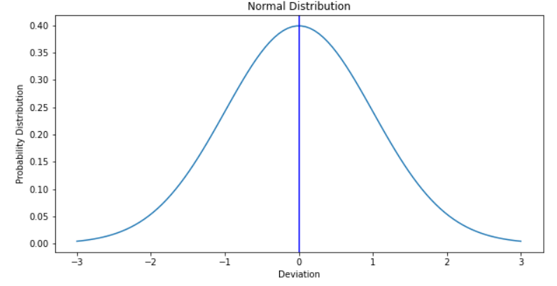
We assume that the natural processes ( manufacturing processes, population height) are normally distributed. Process Variance and Standard deviations are inputs for the Normal Distribution Curve shown above.
5. Variance
It measures the spread in the observed values. In other words, variance determines how far the given values are from the mean.
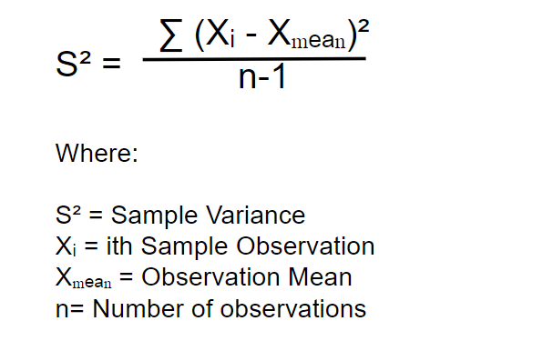
6. Standard Deviation
Similar to variance, standard deviation also measures the spread in the observed values. In other words, it determines how far the given values are from the mean.
Mathematically standard deviation is equal to the square root of variance.
Standard Deviation (σ) = √ Variance (S²)
- The higher the difference between the observed value and the mean, Higher will be the Standard Deviation.
- It measures the process capability.
- The standard deviation unit is the same as the measured data. For example, the standard deviation of a diameter in mm will be in mm.
How to measure Process Capability indices (Cp & Cpk)?
Cp and Cpk are process capability indices used to measure Normal Distributed Process Capability. Note that, Process Capability Indices (Cp and Cpk) apply to Statistically controlled normally distributed processes only.
What is the Difference between Cp, Cpk and Pp, PPk?
We also use terms Pp (Preliminary Process Capability) and Ppk (Preliminary Process Capability Index) to evaluate new processes where we do not have enough data to prove that the process is in statistical control.
We can say the process is statistically controlled when Pp and Ppk values becomes equal to Cp and Cpk respectively.
Assumptions during Process Capability Calculations
We consider the following assumptions while calculating the process capability indices:
- The process is statistically Controlled.
- The process is following Normal Distribution.
- Sample data represents the whole population.
- Sample Data is random.
Process Capability (Cp)
Cp value determines if our process is capable of manufacturing parts within specifications.
Process Capability (Cp) Calculation Formula
Mathematically Cp is equal to the ratio of the Specification Limit and Process Limit.
Cp = Specification Limit / Process Limit
= (USL – LSL) / 6σ
We can conclude the following points from the above calculation formula for Process Capability.
- We can consider a process capable if Cp ≥ 1.
- When Cp < 1: Some of the manufactured parts are out of specification limit.
- We can make a process more capable by increasing the specification limits or reducing process limits. An increase in Process limits will increase the product cost. Therefore it is recommended to optimize specification limits to improve the process capability.
- Cp gives no information on if the process is centered to mean or not.
Process Capability Index (Cpk)
Cpk or Process Capability Index determines if our process is in the center of the specification limits.
Process Capability (Cpk) Calculation Formula
Mathematically Cpk is equal to the minimum of the difference between USL / LSC and mean divided by 3 times of standard deviation.
Cpk = min [ ( USL – μ ) / 3σ, ( μ – LSL ) / 3σ ]
Where μ = mean
We can also calculate Cpk from the Cp.
Cpk = Cp ( 1 – k )
where
k = |(m-µ)| / [ ( USL – LSL ) ] / 2
m = ( USL + LSL ) / 2
0 ≤ k ≤ 1
We can conclude the following points from the above calculation formula for the Process Capability index.
- Cpk overcomes the limitations of Cp. It determines if the process is centered.
- Since the k value varies from 0 to 1, Cpk can be less than or equal to Cp.
Capability Ratio Cr
Capability Ratio is inverse of the process capability (Cp)
Cp = 1 / Process Capability (Cp)
= 6σ / (USL – LSL)
If
Cr < 0.75 : The process is capable.
0.75 ≤ Cr ≤1.00 : the process is capable with tight control.
Cr >1 : the process is not capable.
Cp and Cpk Calculator
You can also use our calculator to calculate the Cp and Cpk values from the upper specification limit (USL), lower specification limit (LSL), standard deviation(σ), and process mean(μ).
Understanding Cp & Cpk using Bell Curve
We can use the bell curve effectively to understand the process and get actionable insights.
When the Process is Centric
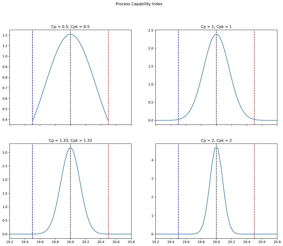
We can conclude the following points from the above bell curves for a fully centric process.
- The Cp and Cpk values are equal for a fully centric process.
- The manufacturing or assembly process width reduces with an increase in the value of the process capability index.
- A Higher Cp value indicates higher process capability.
When the Process is not centric
Let’s consider an example of a 4σ capable process to understand how Cp and Cpk value gives insight into the process.
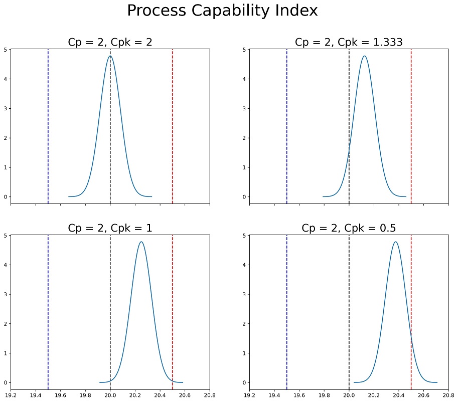
We can conclude the following points from the above bell curves for a non-centric normal distributed process.
- All of the above processes are highly capable. But they are shifted from the center.
- Cp tells us about the process capability only. It gives no information about process behavior in comparison to Specification Limits.
- Cpk value reduces as the process starts shifting from nominal.
- When Cp=2 and Cpk= 2, the process is capable and centric.
- When Cp=2 and Cpk= 0.5, the process is capable but shifted from the mean.
Process Capability Index and Process Stability
We can determine a process behavior by analyzing Process Capability Index (Cp and Cpk) values.
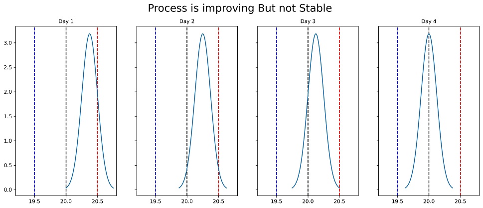
The above image shows an improved but unstable process. Here day by day the process is improving. Here we do not have enough data. The process stabilized on day 4, but we are unsure if it will stop here or will continue moving towards the left.
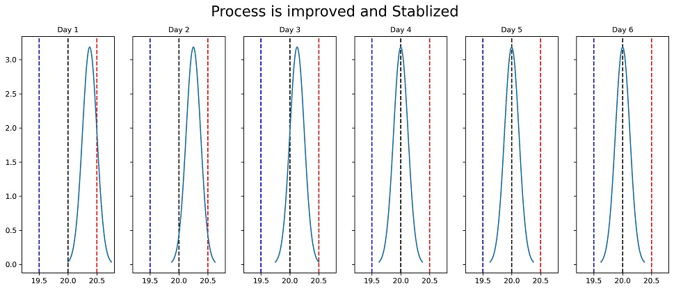
The above image shows a improved and stable process. Day by day the process is improving and stabilizing for a certain time.
Cpk and Rejection Rate (ppm)
We can determine the number of rejected parts per million from Cpk values for a normally distributed process. The following table indicates the parts per million rejection and standard deviation against Cpk values.
| Cpk | Sigma | ppm |
|---|---|---|
| 0.5 | 1.5 | 1,33,610 |
| 1 | 3 | 2,700 |
| 1.33 | 4 | 64 |
| 2 | 6 | 0.00198 |
The above table indicates 64 parts will be out of specification limits if our process is 4σ capable and Cpk = 1.33. Therefore, we can predict the rejected parts per million of manufactured parts through statistical analysis of a normally distributed process.
To sum up, the Process Capability index (Cp & Cpk) is a statistical measure of a normally distributed process’s ability to produce parts within specified limits.
We suggest you also read this article on tolerance stack-up analysis.
Add a Comment